· 17 min read
Technical Challenges of Indirect Control Flow
Abstract
This article discusses the challenges any binary analysis framework will face with indirect control flow. It covers indirect calls, jump tables (indirect jumps), and comments upon existing approaches as well as our techniques. We also touch upon a few other interesting topics such as noreturn analysis, side channel attack mitigations (retpoline), and compiler optimizations.
A wide range of jump table binaries can be found on our open source repository bintests.
Introduction
Any form of compiled binary analysis, binary rewriting, post-compilation optimization, obfuscation, deobfuscation, etc will face the challenge of making sense of indirect control flow. For the purpose of this article we will focus solely on x86 contained inside of PE files generated by a compiler. Typically control flow represents itself in the form of concrete branch statements, returns, and calls. However there are times when indirect control flow must be performed. Such is the case with unknown call targets at compile time.
Stability is a direct tradeoff for more risky interpretations of indirect control flow. Depending on the goals of a binary analysis project different approaches are suitable. When we designed BLARE, we made it a hard set rule to not trade stability for coverage. On the other hand, programs such as IDA Pro, Ghidra, and Binary Ninja are more tolerant of misinterpretation of indirect control flow as it is expected that the user can spot and correct the errors. Obviously the creators of these analysis tools have invested greatly in properly handling indirect control flow, however at the end of the day it is not catastrophic if misinterpretation occurs for analysis tools. This however is not the case for binary rewriting. A misinterpretation of an indirect call or jump table could introduce instability, cause binaries to crash, and cost companies money and engineering time to rectify the issue. We have invested heavily into making our framework as stable as possible and would like to share some of our research with the public.
1.0 - Indirect Calls
Any compiled binary with imports to library routines will contain indirect control flow. In the PE file there is a data directory called the IAT (Import Address Table) which will contain the addresses of imported routines for which the windows loader resolves for you. The compiler will emit call instructions to import thunks or call instructions which directly dereference the IAT.
call QWORD PTR [rip+0x1048] ; IAT!QueryPerformanceCounterIndirect calls to imports are very trivial to handle as the destination can be inferred if the memory location referenced by the operand lands within the IAT range. If there is no desire to understand the destination of indirect calls one might think to simply continue disassembling the instruction(s) after the call. However this is actually unstable and not a proper approach for disassembly in our opinion. Why? Because if the indirect call is invoking a non-returning function that the compiler is aware of then optimizations will be performed to omit any further instructions after the call instruction. Therefore if you simply advance the disassembler past the indirect call and attempt to disassemble there will be situations where the instructions are data or part of another function. At best you will have an incorrect control flow graph, and at worst you will begin to disassemble at misaligned instruction boundaries and interpret data such as jump tables as instructions leading to non-fatal disassembly but catastrophic results after obfuscation is applied.
Google’s Project Syzygy acknowledges this issue and attempts to enhance stability by tracking known imports that do not return. Although this approach is not foolproof, they also try to determine if a call is to a non-returning subroutine by parsing the bytes following the call. Compilers frequently insert int3, ud2, and nop instructions of varying lengths after non-returning call instructions. The int3 and ud2 instructions are used to catch if execution returns, while nop instructions are used for alignment purposes. However, each compiler handles this differently. Our framework addresses this challenging issue with custom in-house solutions. We build on and enhance Syzygy’s approach, achieving stability sufficient to rewrite over 97% of Chrome, 99% of Unreal Engine games, 98% of IL2CPP Unity Engine games, and over 95% of Windows components, such as ntoskrnl, win32k modules, ntdll, and Hyper-V (hvix64/hvax64).
Our algorithm to determine if a function returns or not simply examines the terminators of basic blocks. If all basic block terminators are interrupts (such as fastfails) or calls to other known non-returning functions, the function can be said to not return. Our initial approach was over-approximating, which led to an interesting edge case in Microsoft’s Hyper-V module hvix64.exe, containing the Intel hypervisor variant of Hyper-V. The function retpoline_trampoline, shown in Figure 2, was initially determined to be non-returning.
retpoline_trampoline is a countermeasure to speculative execution attacks. You can read more about these attacks and mitigations here and here.
Our misattribution resulted in every call to retpoline_trampoline (and thus every indirect call) being classified as non-returning. Consequently, B.L.A.R.E.’s disassembler would not continue disassembling after the call, leading to the premature termination of functions. The functionality at address 0xFFFFF8000023CA2C in Figure 2 clearly alters the return destination. Although it conflicts with CET (Control-flow Enforcement Technology), this version of hvix64 is somewhat outdated. The revised noreturn analysis algorithm is now more conservative in its judgment and properly handles this function.
.text:FFFFF8000023CA20 retpoline_trampoline proc near
.text:FFFFF8000023CA20                 call    loc_FFFFF8000023CA2C
.text:FFFFF8000023CA25 ; ------------------------------------------------
.text:FFFFF8000023CA25 loc_FFFFF8000023CA25:
.text:FFFFF8000023CA25                 pause
.text:FFFFF8000023CA27                 lfence
.text:FFFFF8000023CA2A                 jmp     short loc_FFFFF8000023CA25
.text:FFFFF8000023CA2C ; ------------------------------------------------
.text:FFFFF8000023CA2C loc_FFFFF8000023CA2C:
.text:FFFFF8000023CA2C                 mov     [rsp+0], rax
.text:FFFFF8000023CA30                 retn
.text:FFFFF8000023CA30 retpoline_trampoline endp1.1 - Indirect Unconditional Jumps
In addition to indirect calls, x86 has indirect branches. Determining the target locations can be quite a challenge when they aren’t, for example, just loading an address from the IAT. Especially those with computed addresses for which control flow will be transferred to. A great example of these are jump tables. Jump tables are compile-time generated tables of target addresses. At runtime control flow is transferred by indexing into this table of addresses and jumping to the selected address. From a disassembler’s perspective a sequence of instructions will look as follows in Figure 3. The question is where do you go after the “jmp rax”? It’s obvious you can’t just advance the instruction pointer and continue disassembling. Even if the instructions following the jmp are aligned, proper basic block boundaries won’t be formed unless all the targets of the jump table are identified. For the purpose of this article we will only talk about indirect jumps in reference to jump tables but they are prevalent in many forms of obfuscation such as control flow flattening and virtual machine based obfuscation.
lea     rcx, jpt_1400050D4
movsxd  rax, dword ptr [rcx+rax*4]
add     rax, rcx
jmp     rax

jpt_1400050D4   dd offset loc_1400050D6 - 140005138h
                dd offset loc_140005103 - 140005138h
                dd offset loc_1400050E8 - 140005138h
                dd offset loc_1400050F1 - 140005138h
                dd offset loc_1400050DF - 140005138h
                dd offset loc_14000510C - 140005138h
                dd offset loc_140005115 - 140005138h
dd offset loc_1400050FA - 140005138h1.2 - Jump Table Variants
Compilers implement jump tables in various ways. When executables are relocatable, virtual addresses must be computed either at runtime or load time using relocations. However, since jump tables are generated during compilation, additional instructions must be inserted into the instruction stream to compute the target virtual addresses. Furthermore, 32-bit and 64-bit variants of jump tables introduce additional complexity. 32-bit relocatable code relies heavily on PE relocations due to the absence of instruction pointer (IP) relative addressing. For 32-bit code, jump tables are relatively straightforward and consist of an array of PE relocations to each target block. An example of a 32bit jump table can be seen below in Figure 4.
; Relocations are present at each 4 byte value
.rdata:0040216C jpt_4040AC      dd offset loc_4040E9
.rdata:0040216C                 dd offset loc_4040B3
.rdata:0040216C                 dd offset loc_4040C1
.rdata:0040216C                 dd offset loc_4040C8
.rdata:0040216C                 dd offset loc_4040BA
.rdata:0040216C                 dd offset loc_4040D6
.rdata:0040216C                 dd offset loc_4040DD
.rdata:0040216C dd offset loc_4040CFHowever 64bit jump tables tend to be a bit more complex. Instead of encoding absolute addresses in the tables, the latest LLVM and MSVC emit tables filled with relative addresses. LLVM uses the binary relative address of the table itself in combination with the selected table entry to compute the virtual address of the target destination (Figure 5). Whereas MSVC uses the base address of the module in combination with the jump table entry (an RVA) to compute the virtual address of the jump destination (Figure 6). The benefit to this is that encoded table entries only need to be 4 bytes in size but can still be used to compute 8 byte addresses.
lea     rcx, jpt_1400050D4
movsxd  rax, dword ptr [rcx+rax*4]
add     rax, rcx
jmp raxlea rdx, cs:140000000h
cdqe
mov ecx, [rdx+rax*4+1198h]
add rcx, rdx
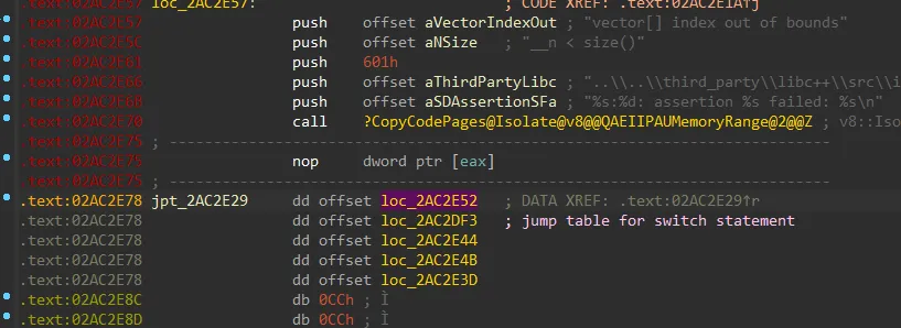
jmp rcxJump tables can also be multi level. In an effort to save even more space when encoding large tables for switch statements with more sparse integer cases, MSVC adds an additional layer of abstraction in the form of another table. These are commonly referred to as “indirect jump tables” but can also be called “multi level jump tables”.
lea     rdx, cs:140000000h
cdqe
movzx   eax, byte ptr [rdx+rax+120Ch] ; Load of Indirect table entry
mov     ecx, [rdx+rax*4+11D4h]        ; Load of Branch Target Table entry
add     rcx, rdx
jmp     rcx

jpt_14000113C   dd offset loc_14000113E - 140000000h
                dd offset loc_140001147 - 140000000h
                dd offset loc_140001150 - 140000000h
                dd offset loc_140001159 - 140000000h
                dd offset loc_140001162 - 140000000h
                dd offset loc_14000116B - 140000000h
                dd offset loc_140001174 - 140000000h
                dd offset loc_14000117D - 140000000h
                dd offset loc_140001186 - 140000000h
                dd offset loc_14000118F - 140000000h
                dd offset loc_140001198 - 140000000h
                dd offset loc_1400011A1 - 140000000h
                dd offset loc_1400011AA - 140000000h
                dd offset def_14000113C - 140000000h
byte_14000120C  db 0, 0Dh, 0Dh, 0Dh, 0Dh, 0Dh, 0Dh, 0Dh, 0Dh, 0Dh, 0Dh
                db 0Dh, 0Dh, 0Dh, 0Dh, 0Dh, 0Dh, 0Dh, 0Dh, 0Dh, 1, 0Dh
                db 0Dh, 0Dh, 0Dh, 0Dh, 0Dh, 0Dh, 0Dh, 0Dh, 0Dh, 0Dh, 0Dh
                db 0Dh, 0Dh, 0Dh, 0Dh, 0Dh, 0Dh, 0Dh, 2, 0Dh, 0Dh, 0Dh
                db 0Dh, 0Dh, 0Dh, 0Dh, 0Dh, 0Dh, 0Dh, 0Dh, 0Dh, 0Dh, 0Dh
                db 0Dh, 0Dh, 0Dh, 0Dh, 0Dh, 3, 0Dh, 0Dh, 0Dh, 0Dh, 0Dh
                db 0Dh, 0Dh, 0Dh, 0Dh, 0Dh, 0Dh, 0Dh, 0Dh, 0Dh, 0Dh, 0Dh
                db 0Dh, 0Dh, 0Dh, 4, 0Dh, 0Dh, 0Dh, 0Dh, 0Dh, 0Dh, 0Dh
                db 0Dh, 0Dh, 0Dh, 0Dh, 0Dh, 0Dh, 0Dh, 0Dh, 0Dh, 0Dh, 0Dh
                db 0Dh, 5, 0Dh, 0Dh, 0Dh, 0Dh, 0Dh, 0Dh, 0Dh, 0Dh, 0Dh
                db 0Dh, 0Dh, 0Dh, 0Dh, 0Dh, 0Dh, 0Dh, 0Dh, 0Dh, 0Dh, 6
                db 0Dh, 0Dh, 0Dh, 0Dh, 0Dh, 0Dh, 0Dh, 0Dh, 0Dh, 0Dh, 0Dh
                db 0Dh, 0Dh, 0Dh, 0Dh, 0Dh, 0Dh, 0Dh, 0Dh, 7, 0Dh, 0Dh
                db 0Dh, 0Dh, 0Dh, 0Dh, 0Dh, 0Dh, 0Dh, 0Dh, 0Dh, 0Dh, 0Dh
                db 0Dh, 0Dh, 0Dh, 0Dh, 0Dh, 0Dh, 8, 0Dh, 0Dh, 0Dh, 0Dh
                db 0Dh, 0Dh, 0Dh, 0Dh, 0Dh, 0Dh, 0Dh, 0Dh, 0Dh, 0Dh, 0Dh
                db 0Dh, 0Dh, 0Dh, 0Dh, 9, 0Dh, 0Dh, 0Dh, 0Dh, 0Dh, 0Dh
                db 0Dh, 0Dh, 0Dh, 0Dh, 0Dh, 0Dh, 0Dh, 0Dh, 0Dh, 0Dh, 0Dh
                db 0Dh, 0Dh, 0Ah, 0Dh, 0Dh, 0Dh, 0Dh, 0Dh, 0Dh, 0Dh, 0Dh
                db 0Dh, 0Dh, 0Dh, 0Dh, 0Dh, 0Dh, 0Dh, 0Dh, 0Dh, 0Dh, 0Dh
                db 0Bh, 0Dh, 0Dh, 0Dh, 0Dh, 0Dh, 0Dh, 0Dh, 0Dh, 0Dh, 0Dh
db 0Dh, 0Dh, 0Dh, 0Dh, 0Dh, 0Dh, 0Dh, 0Dh, 0Dh, 0Ch1.3 - Jump Table Boundedness
Now is probably a good time to discuss the topic of boundedness. Most jump tables have bounds to them which can be obtained by analysis of the native instructions. In Figure 8 we clearly depict boundedness in an LLVM 64bit jump table. However, not all jump tables have such easily identifiable bounds to them. If the compiler is made aware of all possible values used to derive the jump table entry, or it believes that index sanitization is not required, it can omit a bounds check on the table index value. Such is the common case for lots of code generated by the Rust compiler. In Rust there is a concept called “matching”. The compiler can safely omit bounds checking more often as all branch destinations are known at compile time. The equivalent in MSVC C is to use the intrinsic __assume(0) which tells the compiler that the current sequence of instructions is unreachable. It is very difficult to handle unbounded jump tables. You cannot over approximate the number of jump table entries otherwise you will misinterpret arbitrary bytes as jump table entries and thus your disassembler will become misaligned.
Here’s a neat example of boundedness in godbolt, try commenting out the default case containing __assume(0) and see how the emitted code changes.
;
; Fetch and compare bounds
;
mov     eax, [rsp+38h+var_18] ; Fetch Index
dec     eax                   ; Normalize Index
cmp     eax, 0F0h             ; Bounds compare
ja      def_14000113C         ; If index is greater than the bound
;
; Jump table dispatch
;
lea     rdx, cs:140000000h
cdqe
movzx   eax, byte ptr [rdx+rax+120Ch]
mov     ecx, [rdx+rax*4+11D4h]
add     rcx, rdx
jmp rcx1.3 - The Ill Fated “Guess & Check”
You might think you can get away with guessing and checking entries in jump tables by looping every 4 bytes, interpreting each as an entry, and then validating if the address computed is instruction-aligned, located in executable memory, and guarded by the same exception information as the indirect jump itself. However, this is unsafe. A simple counter-example would be jump tables that reside directly after one another, without some sort of bound, it is impossible to know where one table ends and another begins.. As it turns out, jump tables residing directly after one another is actually very common. On MSVC, we observed that any function which has nested jump tables will have the tables placed directly after one another. As a result, we quickly ruled out using the guess and check method as B.L.A.R.E.’s primary goal is stability.
.rdata:E300B8 jpt_5D7DAE  dd offset loc_5D7DB0 - 0E300B8h
.rdata:E300B8             dd offset loc_5D7FC0 - 0E300B8h
.rdata:E300B8             dd offset loc_5D81D0 - 0E300B8h
.rdata:E300B8             dd offset loc_5D83E0 - 0E300B8h
.rdata:E300B8             dd offset loc_5D85F0 - 0E300B8h
.rdata:E300B8             dd offset loc_5D868C - 0E300B8h
.rdata:E300B8             dd offset loc_5D8898 - 0E300B8h
.rdata:E300B8             dd offset loc_5D8AA4 - 0E300B8h
.rdata:E300B8             dd offset loc_5D8CB0 - 0E300B8h
.rdata:E300B8             dd offset loc_5D8E88 - 0E300B8h
.rdata:E300B8             dd offset loc_5D9060 - 0E300B8h
.rdata:E300B8             dd offset loc_5D9238 - 0E300B8h
.rdata:E300B8             dd offset loc_5D9410 - 0E300B8h
.rdata:E300B8             dd offset loc_5D95E8 - 0E300B8h
.rdata:E300B8             dd offset loc_5D97C0 - 0E300B8h
.rdata:E300B8             dd offset loc_5D9998 - 0E300B8h
.rdata:E300F8 jpt_5D9BFB  dd offset loc_5D9C00 - 0E300F8h
.rdata:E300F8             dd offset loc_5D9D0C - 0E300F8h
.rdata:E300F8             dd offset loc_5D9E18 - 0E300F8h
.rdata:E300F8             dd offset loc_5D9F24 - 0E300F8h
.rdata:E300F8             dd offset loc_5DA030 - 0E300F8h
.rdata:E300F8             dd offset loc_5DA164 - 0E300F8h
.rdata:E300F8             dd offset loc_5DA298 - 0E300F8h
.rdata:E300F8             dd offset loc_5DA3CC - 0E300F8h
.rdata:E300F8             dd offset loc_5DA500 - 0E300F8h
We advise against approaching the issue of jump table bounds using the approaches outlined above as it is not viable on any decently complex binary. In the next section, we present a more stable approach to determine the targets of jump tables using subgraph isomorphism.
1.4 - Jump Table Analysis
Currently our efforts are fully invested in x86. This will change in the future as we grow. For the time being we approach the jump table analysis as a subgraph isomorphism problem. To begin, we create a DAG from use-definitions of native registers. We can then compare pre-defined jump table DAGs to one constructed from our haystack of disassembled instructions. Figure 9 depicts an example of a haystack DAG. The structure of the DAG represents how registers are used between instructions. Using a DAG also allows for instruction ordering deviations.
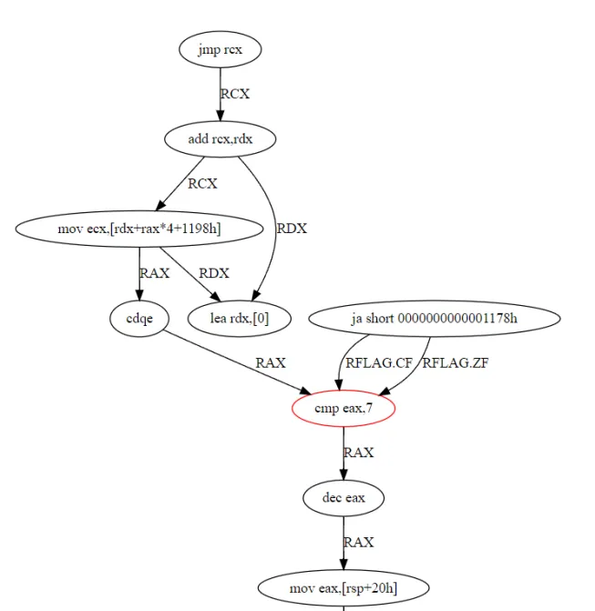
We perform several micro-optimizations to reduce the number of predefined DAGs required. For instance, in our node comparison lambda, we treat move and any sign-extended move variants as equivalent. This approach accommodates minor variations within the jump table code without necessitating numerous DAG implementations. You may have noticed the fact that the CMP instruction in Figure 9 seems to have a flow edge leaving from it despite it not actually producing a register value. We have made a use case specific micro-optimization to our DAG creation algorithm to change the semantics of the CMP instruction. We make the CMP instruction act as though it writes to the register operand as if it was a SUB. The reason for this optimization is simple; we do not care where the register is set which contains the index (in the CMP), we only care that a bound exists. This micro-optimization puts less requirements on the haystack and disassembler. To reiterate, the “dec eax” and “mov eax, [rsp+0x20]” in figure 8 have no useful contribution to identifying the jump table variant.
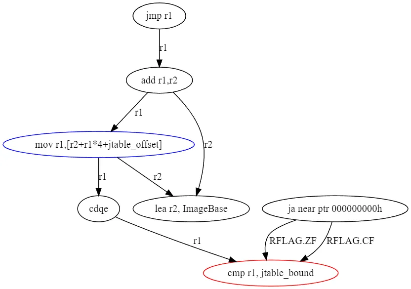
The algorithm used for subgraph isomorphism (VF2) is implemented by petgraph, a rust graph library which we highly recommend. When the algorithm finds a match it returns a mapping of node indices to the pattern DAG. This allows us to write extractor algorithms to properly handle jump table variants. For example if we match a 64bit MSVC jump table then we know which instruction contains the bounds, we know how to interpret the table, and thus we can parse the jump table. Figure 10 depicts our MSVC 64bit jump table predefined DAG, the node with a red outline is the bound node, the node with the blue outline is the jump table index operation.
The petgraph subgraph isomorphism algorithm enables us to specify custom functions for comparing edges and nodes. We do not need to compare edges because the graph’s structure inherently defines register usage (the DAG is made up of use-definition chains). However, special care is required when comparing nodes, as instructions can vary significantly based on the compiler’s choices. Constant values and IP-relative encoded memory operands are excluded from node comparison. Additionally, registers are not used in the comparison function since the register allocator may select different registers than those in our predefined DAGs. To emphasize, the graph’s structure already dictates register usage, so there is no need to compare register usage during node comparison.
With a limited set of pre-defined DAGs, we can parse the vast majority of 64-bit and 32-bit jump tables. Adding more pre-defined jump table DAGs to our framework is straightforward, requiring only the use of Rust macros we have already developed.
1.5 - Limitations
As stated at the beginning of this article, the requirements of indirect control flow analysis are dependent on the project goals. For us stability is extremely important. Therefore we believe we have produced an adequate solution that allows us to understand the vast majority of jump tables without compromising stability. Our approach is fast, easy to understand, and extendable.
However, it has its limitations, most notably the lack of support for unbounded jump tables. While these are typically rare in C and C++ code, they are much more common in code generated by Rust. The Rust compiler excels in compile-time analysis as a result of its strict type system, bounds checking, known-bit-analysis, etc. The compiler is able to understand which code is reachable and which is not, allowing it to eliminate the need for bounds checking in most jump tables.
Another limitation is that our DAG comparison algorithm does not check the semantical usage of registers within individual instructions themselves. Although the structure of the DAG defines register use and definition at the instruction level granularity it does not convey how the register is used within the instruction itself. This is a noteworthy distinction as it is theoretically possible to trick our DAG patterns by simply rearranging the register usage inside of a memory operand. Both of the below instructions would create the same edges in a use-definition DAG graph although there are semantic differences within the instructions themselves. We accept this possibility but treat it as a non-issue for the purpose of jump table analysis.
mov rax, [rsp+r10*4]
; vs
mov rax, [r10+rsp*4]
Lastly, while our jump table analysis solution may not identify every single jump table, it is designed to safely handle scenarios where some may be unidentifiable. CodeDefender employs partial binary rewriting, meaning that not all code in the binary file is expected to be rewritten. We focus on functions we can fully uncover and understand, avoiding manipulation of those we cannot. This emphasis on stability ensures that our framework and obfuscation remain exceptionally reliable.